Postgres Internals: How Postgres Stores and Retrieves Your Data
Do you ever wonder what happens between the moment you execute your query and when you get your results? Postgres query execution is a beautifully orchestrated process that involves parsing, planning, and execution, with the query planner making critical decisions about how to retrieve your data efficiently.
In this post, I'm going to show you how this works behind the scenes. But to understand how Postgres retrieves data, we first need to understand how it stores data, and the two are more connected than you might think.
A Simple Users Table
Let's keep everything simple. Imagine we have a basic users table, that has this structure:
CREATE TABLE users (
  id       SERIAL PRIMARY KEY,
  username VARCHAR(50) UNIQUE NOT NULL
);

CREATE INDEX index_users_username ON users (username);
We are going to use this users table to break down inner Postgres mechanisms.
1. How Postgres Stores Data on Disk
Before we get into the details of how Postgres fetches data, we should first look at how that data is actually stored on disk. Understanding the storage method is crucial for figuring out why some queries are slow even when you have the right indexes in place.
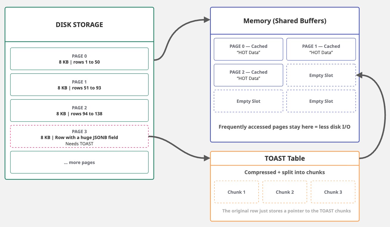
Postgres uses 8192-byte (8 KB) fixed-size blocks, known as pages, for data storage. This size works well with operating system page sizes (usually 4 KB) and disk sector sizes, providing a good balance between I/O efficiency and space. It's configurable at compile time, but almost nobody changes it.
These 8 KB pages have a limitation: tuples (or rows) can't be split across multiple pages. This presents a problem when dealing with large field values, such as TEXT, JSONB, or bytea.
To mitigate this, Postgres uses TOAST (The Oversized-Attribute Storage Technique), which compresses and breaks large fields into smaller chunks, subsequently storing them in a separate TOAST table.
This 8 KB page size allows Postgres to be efficient in most cases. When it reads data from disk, it reads entire pages. When it writes data, it writes entire pages. Since pages are fixed-size blocks, Postgres can efficiently cache frequently accessed ones in shared buffers, reducing disk I/O.
2. The Three Forks: Heap, FSM, and Visibility Map
As we know, Postgres uses 8 KB pages, a design choice that achieves a balance between efficiency and storage. However, not all pages are equal. A single table has three page types (or forks), each stored in separate files: heap pages, which hold your actual row data; FSM pages, which track the free table space; and VM pages, which manage row visibility at page level. While they all share the same 8 KB structure, the contents of each are entirely different.
| Page/Fork | File Suffix | Purpose |
|---|---|---|
| Main | Heap pages containing actual row data | |
| FSM | _fsm |
Free Space Map — tracks free space in each page |
| VM | _vm |
Visibility Map — tracks which pages are fully visible |
Heap Pages store the actual table rows. We're going to discuss these in detail in the next section.
Free space map (FSM) pages are used to track and locate available space within a table or a index.
Postgres uses these to efficiently reuse space for inserts and updates, reducing table bloat.
FSM pages are updated during INSERT or UPDATE operations and are primarily managed by VACUUM operations.
Visibility maps (VM) are pages related to heap pages that track which pages contain tuples (rows) visible to all active transactions.
These are primarily used during VACUUM and Autovacuum operations.
VMs store two bits per page: the first one (all-visible bit) indicates that every row version on that page is visible to current and future transactions.
The second one (all-frozen bit) indicates if all rows in the page are "frozen," meaning they're old enough so that Postgres no longer needs to track their transaction IDs.
The good part? We can actually look inside these pages.
We can use pageinspect extension to inspect the internal, low-level contents and structures of our users table pages and rows.
CREATE EXTENSION pageinspect;
Let's check our users table disk structure:
blog=# SELECT pg_relation_filepath('users');

pg_relation_filepath
----------------------
 base/461880/461882
(1 row)
The pg_relation_filepath function returns the output relative to the main Postgres data directory: base/{DB_OID}/{REL_FILENODE}. In this case, the database OID is 461880 and the users table filenode is 461882.
The FSM and VM forks are located at 461882_fsm and 461882_vm, respectively.
As we know the physical location of our data, we can now examine the page structure:
❯ ls -la /Users/leonardodarosa/gdk/postgresql/data/base/461880/461882*

-rw-------  1 leonardodarosa  staff   8192 Jan  7 19:38 /Users/leonardodarosa/gdk/postgresql/data/base/461880/461882
-rw-------  1 leonardodarosa  staff  24576 Jan  7 19:39 /Users/leonardodarosa/gdk/postgresql/data/base/461880/461882_fsm
-rw-------  1 leonardodarosa  staff   8192 Jan  7 19:39 /Users/leonardodarosa/gdk/postgresql/data/base/461880/461882_vm
We can interpret this as: base/my_database/users, base/my_database/users_fsm, and base/my_database/users_vm.
We can do the same for the index_users_username index:
blog=# SELECT pg_relation_filepath('index_users_username');

pg_relation_filepath
----------------------
 base/461880/461890
(1 row)
For the users table, we have the following structure:
$PGDATA/base/461880/
├── 461882      Users Main (heap pages with row data)
├── 461882_fsm  Users Free Space Map (FSM)
└── 461882_vm   Users Visibility Map (VM)
|
├── 461890      index_users_username index
├── 461890_fsm Visibility MapFSM or VM files right after table creation.
Instead, Postgres waits until it's necessary to have them. You might need to run VACUUM first or simply populate the table with enough data for those files to be created.
Each fork is essentially a sequence of 8 KB pages. The main fork contains your data. The FSM and VM are smaller files that track the metadata associated to each the heap page.
2.1 Anatomy of Heap Pages
Heap pages store the actual table rows. Each page has a fixed structure:
| Section | Size | Description |
|---|---|---|
| Page Header | 24 bytes | Metadata: LSN (WAL position), checksum, flags, and pointers to free space. |
| Line Pointers | 4 bytes each |
Array of pointers to tuples. Each entry has the offset and length of a tuple. New pointers are added at the end. |
| Free Space | Variable | Empty space between line pointers and tuples. Shrinks as data is added. |
| Tuples (rows) | Variable | Actual row data. Each tuple has a 23-byte header (xmin, xmax, ctid, etc.), optional null bitmap, and column values. |
| Special Space | 0 bytes | Used by indexes for extra metadata. Empty for heap pages. |
Perfect. Now we know how data is stored on disk and how Postgres structures everything into 8 KB pages. But what's actually inside a tuple? Let's take a closer look at how a row is stored.
3. What Happens During an INSERT
When you execute an INSERT statement, Postgres doesn't immediately write your data to a file. Instead, each row gets a header with internal metadata.
This includes details such as the transaction that created the row, its location within the page, and other flags.
Consider the following statement:
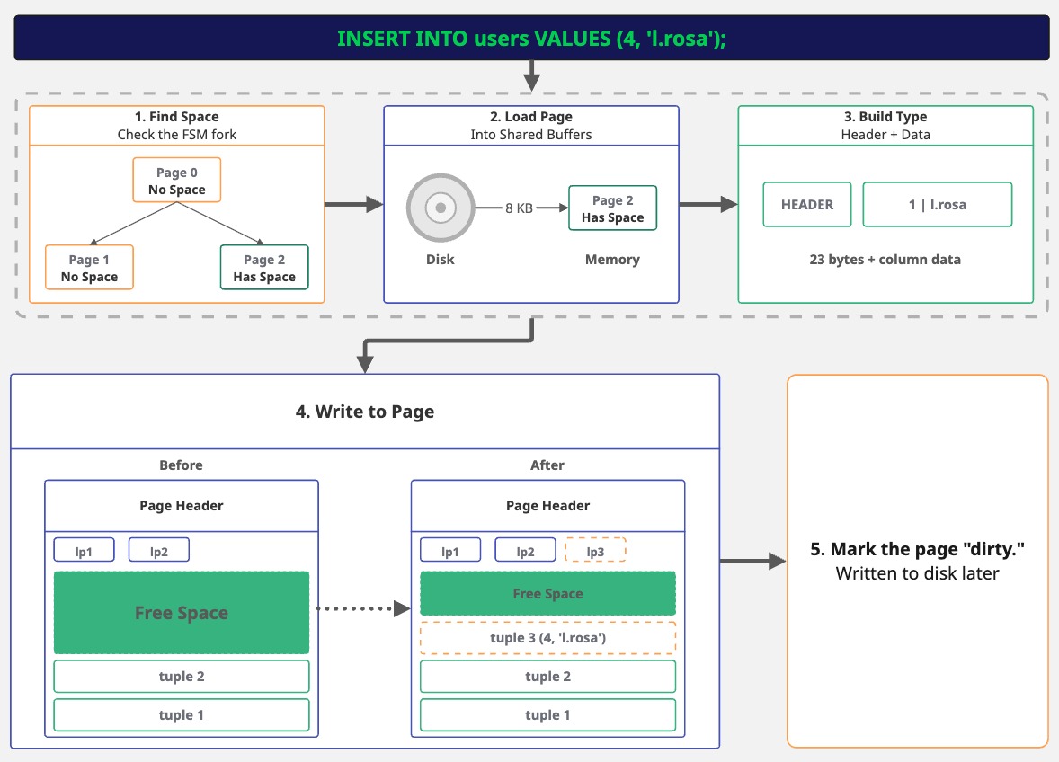
INSERT INTO users (id, username) VALUES (4, 'l.rosa');
When you execute the INSERT statement, Postgres first needs to find space for the row. Remember the FSM fork? Postgres checks it to find a page with enough room for our row. If no page has space, it adds a new one.
Next, it loads the page into memory. If the page isn't already cached, Postgres reads the whole 8 KB page from disk, then it builds the tuple.
Our data, (4, 'l.rosa'), gets a header attached with some internal metadata. The columns, then, are packed as raw bytes.
Now Postgres writes to the page and adds a line pointer (to track where the tuple is) and writes the tuple into the free space.
Finally, the page is marked as "dirty," but it doesn't go to disk right away. This might sound risky, because, what if Postgres crashes? That's precisely where the Write-Ahead Log (WAL) comes in. Before Postgres even alters the page in memory, it writes a record of the change to the WAL. The WAL is sequential and gets flushed to disk immediately on commit. So the change is preserved, even though the actual page write is deferred.
Postgres optimizes performance by batching page writes (during checkpoints). However, the WAL ensures that committed data isn't lost. This "log first, write later" approach is why it's called write-ahead logging.
Let's see what we actually wrote to disk:
SELECT lp, t_ctid, encode(t_data, 'escape') AS readable_data
FROM heap_page_items(get_raw_page('users', 0))
WHERE t_data IS NOT NULL;

 lp | t_ctid |        readable_data
----+--------+-----------------------------
  4 | (0,4)  | \x01\000\000\000\ralice
  5 | (0,5)  | \x02\000\000\000        bob
  6 | (0,6)  | \x03\000\000\000\rmaria
  7 | (0,7)  | \x04\000\000\000\x0Fl.rosa
(4 rows)
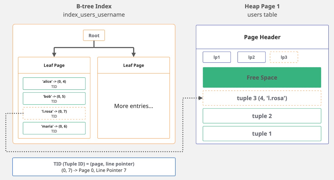
But we're not done yet. Remember we have an index on username? Postgres has to update it too.
It finds the proper position within the B-tree and then adds a new entry.
This entry holds the indexed value, 'l.rosa', along with a pointer, the TID, that directs back to the tuple's location.
Essentially, the index entry looks like this: 'l.rosa' -> (0, 7). The username points to page 0, line 7.
SELECT itemoffset, ctid, data
FROM bt_page_items('index_users_username', 1);

 itemoffset | ctid  |          data
------------+-------+-------------------------
          1 | (0,4) | 0d 61 6c 69 63 65 00 00
          2 | (0,5) | 09 62 6f 62 00 00 00 00
          3 | (0,7) | 0f 6c 2e 72 6f 73 61 00
          4 | (0,6) | 0d 6d 61 72 69 61 00 00
(4 rows)
The ctid is the tuple ID that points to the location of the row in the heap. While index entries are sorted in alphabetical order, the ctid values reflect the order in which the rows were inserted.
That's the whole point of an index: providing sorted access to unsorted data.
INSERT, UPDATE, or DELETE a row, every index on that table gets updated.
If you have five indexes, that's five extra writes for each row change. This is why you should be careful about adding indexes to large tables: they make reading data faster, but slow down writing.
This is why bulk operations can be slow on heavily indexed tables
4. The Query Lifecycle
Now we know how Postgres stores data, through pages, tuples, indexes, all of it. But what happens when we query that data?
When we run SELECT * FROM users WHERE username = 'l.rosa', Postgres processes it through some phases:
| Phase | What it does |
|---|---|
| Parse | checks the syntax, builds parse tree |
| Plan | chooses the best execution strategy |
| Execute | runs the plan, returns results |
4.1 Parse
When Postgres receives your query, it first checks if it's a valid SQL statement. Is the syntax correct? Are the keywords in the right place? If you write SELEC * FROM users, it'll catch the typo here.
After validation, Postgres converts the SQL string into a parse tree, a structured representation it can use internally.
4.2 Plan
Now Postgres has to figure out how to get the data. Should it scan every row (seq scan)? Use an index (index scan, index-only scan)? If there are joins, what's the order? The planner checks the table statistics and available indexes to estimate the cost of different approaches, and it picks the cheapest one.
The query planner uses table statistics to determine things like how many rows we have in the table, how data is distributed, etc.
If the statistics are outdated or inaccurate, the planner can make bad decisions.
That's why you might see a slow query getting faster after running ANALYZE my_table;.
You can check the actual query plan by prepending EXPLAIN to your query.
EXPLAIN shows expected costs based on table statistics without executing the query,
while EXPLAIN ANALYZE actually runs the query and shows real runtime statistics.
EXPLAIN ANALYZE SELECT * FROM users WHERE username = 'l.rosa';
                                           QUERY PLAN
-------------------------------------------------------------------------------------------------
 Seq Scan on users (cost=0.00..1.05 rows=1 width=122) (actual time=0.007..0.007 rows=1 loops=1)
   Filter: ((username)::text = 'l.rosa'::text)
   Rows Removed by Filter: 3
 Planning Time: 0.045 ms
 Execution Time: 0.015 ms
(5 rows)
Something curious happened in the query plan: we have an index on username, but the planner chose a sequential scan (Seq Scan on users) anyway.
Why? The table has just 4 rows sitting in a single page. Reading that one page and checking 4 rows is faster than traversing the B-tree index,
finding the pointer, and then fetching the heap tuple. The planner does the math and picks the less expensive path.
We can compare how the query performs with an index by forcing Postgres to use index_users_username.
We can disable sequential scans for the session with SET enable_seqscan = OFF;:
EXPLAIN ANALYZE SELECT * FROM users WHERE username = 'l.rosa';
                                                          QUERY PLAN
------------------------------------------------------------------------------------------------------------------------------
 Index Scan using index_users_username on users (cost=0.13..2.15 rows=1 width=122) (actual time=0.054..0.055 rows=1 loops=1)
   Index Cond: ((username)::text = 'l.rosa'::text)
 Planning Time: 0.068 ms
 Execution Time: 0.070 ms
(4 rows)
Look at the costs: Seq Scan (0.00..1.05 actual time=0.007..0.007) vs. Index Scan (0.13..2.15 actual time=0.054..0.055).
The index scan is more expensive for this tiny table. And there's a reason why: Seq Scan reads one page, check 4 rows. Done.
Index Scan traverses the B-tree to find 'l.rosa', get the TID (0,7), then fetch the tuple from the heap.
More steps, more overhead.
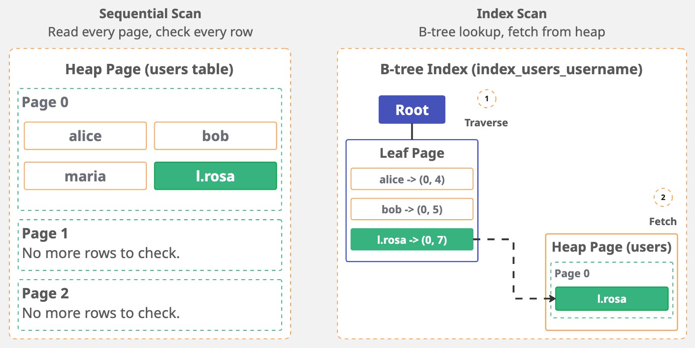
With just 4 rows, an index is unnecessary. However, as the table grows, the equation changes. Scanning each page sequentially becomes a costly operation, and the index starts to make sense.
4.3 Execute
Finally, Postgres runs the plan. But it doesn't process your query in a "top-to-bottom" way. It follows a logical order of execution:
| Order | Clause | What it does |
|---|---|---|
| 1 | FROM/JOIN | Identify source tables, combine rows |
| 2 | WHERE | Filter rows |
| 3 | GROUP BY | group the results |
| 4 | HAVING | filter groups |
| 5 | SELECT | pick columns, evaluate expressions, apply DISTINCT |
| 6 | ORDER BY | Sort the results |
| 7 | LIMIT/OFFSET | Restrict output rows |
For each step, Postgres reads pages from disk (or shared buffers if cached), finds the tuples, checks if they're visible to the current transaction, and returns the results.
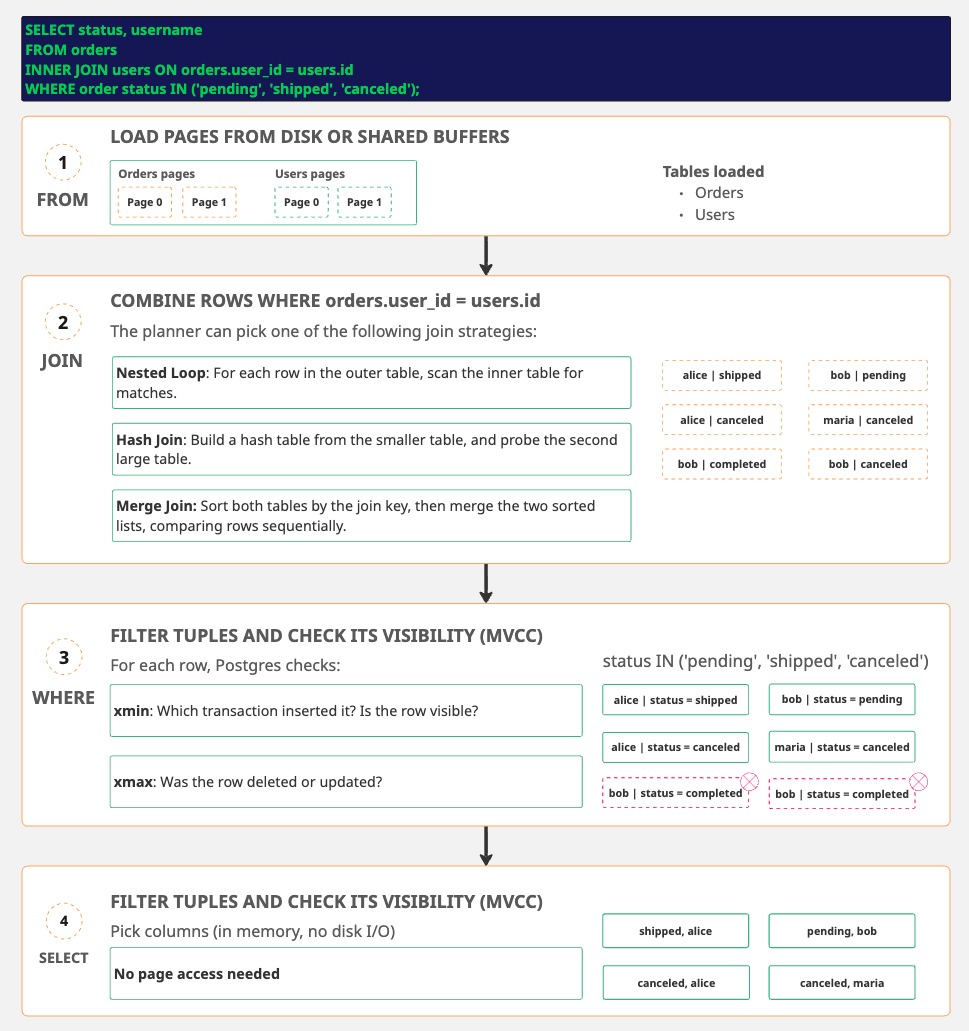
FROM load pages, JOIN may re-access the pages,
WHERE checks the visibility on buffered data, SELECT works in memory.
This execution order also explains a common misconception: some people think that by adding a LIMIT always makes queries fast by fetching only X rows.
It depends. Without an ORDER BY, Postgres can stop early once it has enough rows.
But adding an ORDER BY without a supporting index, makes Postgres to fetch and sort everything before cutting it down to LIMIT X.
-- This is fast, because Postgres can stop after finding the first 10 rows
SELECT * FROM users WHERE active = true LIMIT 10;

-- This is slow, because Postgres has to fetch ALL active users, sorts them, then limit the results
SELECT * FROM users WHERE active = true ORDER BY created_at LIMIT 10;
In the example above, an index on created_at would let Postgres stop early.
It can walk the index in order and quit after 10 rows.